Plot Gower's distance matrix

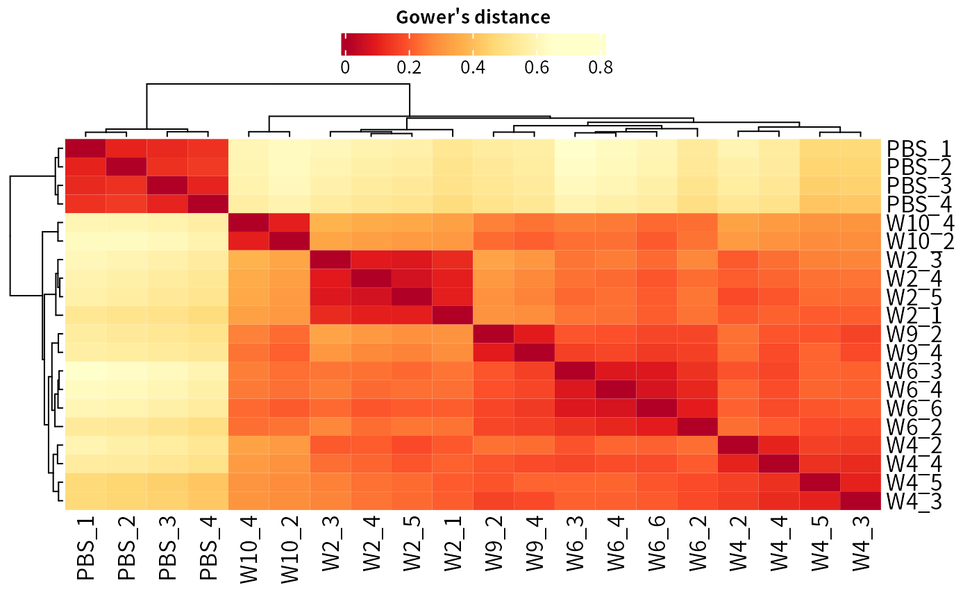
plot_dist generates a distance matrix heatmap using the Gower's distance.

Usage

plot_dist(
  x,
  significant = TRUE,
  pal = "YlOrRd",
  pal_rev = TRUE,
  indicate = NULL,
  font_size = 12,
  plot = TRUE,
  add_values = FALSE,
  value_size = 10,
  digits = 2,
  ...
)

Arguments

x

SummarizedExperiment or DEGdata object, for which differentially expressed/enriched proteins or genes are annotated (output from test_diff() and add_rejections()).

significant

Logical(1), Whether or not to filter for significant proteins.

pal

Character(1), Sets the color panel (from RColorBrewer).

pal_rev

Logical(1), Whether or not to invert the color palette.

indicate

Character, Sets additional annotation on the top of the heatmap based on columns from the experimental design (colData).

font_size

Integer(1), Sets the size of the labels.

plot

Logical(1), If TRUE (default) the distance matrix plot is produced. Otherwise (if FALSE), the data which the distance matrix plot is based on are returned.

add_values

Logical(1). Display the distance value on heatmap.

value_size

Numeric(1). Font size of distance.

digits

Integer(1), indicating the number of decimal places of distance.

...

Additional arguments for Heatmap function as depicted in Heatmap

Value

A heatmap plot (generated by Heatmap)

Examples

# Load example
data(Silicosis_pg)
data <- Silicosis_pg
data_unique <- make_unique(data, "Gene.names", "Protein.IDs", delim = ";")

# Make SummarizedExperiment
ecols <- grep("LFQ.", colnames(data_unique))


## Load experiement design
data(Silicosis_ExpDesign)
exp_design <- Silicosis_ExpDesign
se <- make_se(data_unique, ecols, exp_design)

# Filter and normalize
filt <- filter_se(se, thr = 0, fraction = 0.4, filter_formula = ~ Reverse != "+" & Potential.contaminant!="+")
#> filter base on missing number is <= 0 in at least one condition.
#> filter base on missing number fraction < 0.4 in each row
#> filter base on giving formula 

norm <- normalize_vsn(filt)
#> vsn2: 8762 x 20 matrix (1 stratum). 
#> Please use 'meanSdPlot' to verify the fit.

# Impute missing values using different functions
imputed <- impute(norm, fun = "MinProb", q = 0.05)
#> Imputing along margin 2 (samples/columns).
#> [1] 0.3026531

# Test for differentially expressed proteins
diff <- test_diff(imputed, "control", "PBS")
#> Tested contrasts: W10_vs_PBS, W2_vs_PBS, W4_vs_PBS, W6_vs_PBS, W9_vs_PBS
#> Strimmer's qvalue(t)
dep <- add_rejections(diff, alpha = 0.05, lfc = 1)

# Plot correlation matrix
plot_dist(dep)