Plot the distribution of statistic valuse. develop from statistics_plot

Usage

plot_statistics(
  object,
  statistic = c("diff", "t.stastic", "p.val", "p.adj"),
  contrasts = NULL
)

Arguments

object: A SummarizedExperiment or DEGdata obejct from test_diff / test_diff_deg or add_rejections
statistic: Character, in c("diff","t","p.val","p.adj")
contrasts: Characters or NULL, plot contrasts. If NULL, plot all tested contrasts in objest.

Value

The distribution histogram of statistics

Examples

# Load example
data(Silicosis_pg)
data <- Silicosis_pg
data_unique <- make_unique(data, "Gene.names", "Protein.IDs", delim = ";")

# Differential test
ecols <- grep("LFQ.", colnames(data_unique))
se <- make_se_parse(data_unique, ecols,mode = "delim")
filt <- filter_se(se, thr = 0, fraction = 0.4, filter_formula = ~ Reverse != "+" & Potential.contaminant!="+")
#> filter base on missing number is <= 0 in at least one condition.
#> filter base on missing number fraction < 0.4 in each row
#> filter base on giving formula 
norm <- normalize_vsn(filt)
#> vsn2: 8762 x 20 matrix (1 stratum). 
#> Please use 'meanSdPlot' to verify the fit.
imputed <- impute(norm, fun = "MinProb", q = 0.05)
#> Imputing along margin 2 (samples/columns).
#> [1] 0.3026531
diff <- test_diff(imputed, type = "control", control  = c("PBS"), fdr.type = "Storey's qvalue")
#> Tested contrasts: W10_vs_PBS, W2_vs_PBS, W4_vs_PBS, W6_vs_PBS, W9_vs_PBS
#> Storey's qvalue
dep <- add_rejections(diff, alpha = 0.01,lfc = 2)

# plot statistics distribution
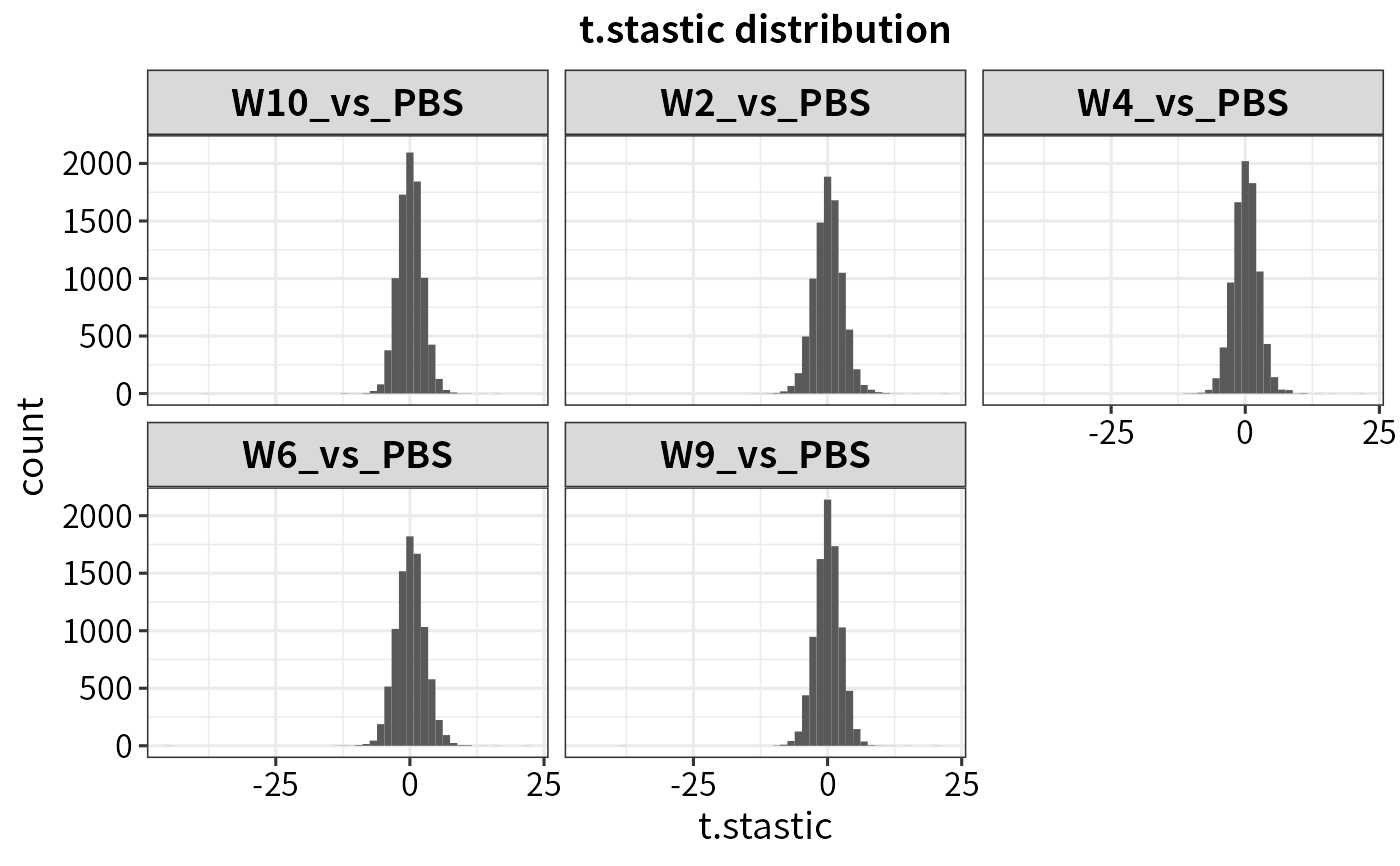
plot_statistics(dep, statistic = "t.stastic")

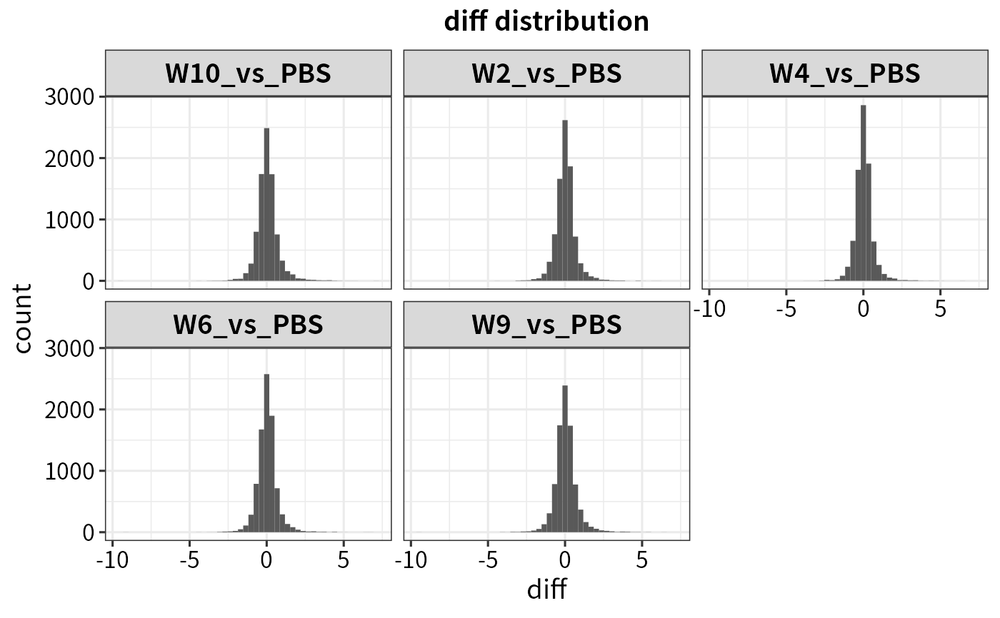
plot_statistics(dep, statistic = "diff")