Quick start
Zhenhuan Feng
01_Quick_start.RmdAbstract
This vignette gives an overview of the DEP2 analysis pipeline.
Introduction
DEP2 provides a differentially expressed/enriched analysis toolkit for mass spectrometry based quantitative proteomics data utilizing the limma package for statistical analysis (Ritchie et al. 2015). DEP2 is an upgraded version of the previous package DEP (Zhang et al. 2018) and provides a comprehensive workflow for proteomics analysis, encompassing data processing, missing value imputation, hypothesis test, visualization and downstream functional exploration.
DEP2 provide three types of differential proteomics analysis:
The pipeline for proteins-level expression/enrichment analysis, starting with protein-level quantity data.
The pipeline for proteins-level expression/enrichment analysis, starting with peptide-level quantity data.
The pipeline for post-translation modification(PTM)-specified proteomics, performed upon modified peptides quantities.
In addition, DEP2 also includes a packaged RNA-seq data analysis pipeline from the DESeq2.
Example Data
In this section, we showcase the utilization of the DEP2 pipelines by employing data from a multiple-omics study of a silicosis mouse model (Wang et al., 2022), which are built-in data in the package. These datasets are included as built-in data within the DEP2 package. Additionally, the data can be accessed in table format from the repository at github.com/mildpiggy/OmicsExample.
## The proteomics data represented in protein-level format (proteingroup.txt output from MaxQuant).
data(Silicosis_pg)

## The proteomics data represented in peptide-level format (peptides.txt output from MaxQuant).
data(Silicosis_peptide)

## Experiment design table providing annotations for the samples.
data(Silicosis_ExpDesign)

## Phosphoproteomics data (Phospho(STY)Sites.txt output from MaxQuant).
data(Silicosis_phos)

## RNA-seq counts data.
data(Silicosis_counts)
Get Start
The four pipelines can be executed step-by-step as outlined below:
Proteingroup Workflow
The conventional workflow starts with protein-level data.
## 1. Construct SummarizedExperiement
unique_pg <- make_unique(Silicosis_pg, names = "Gene.names", ids = "Protein.IDs")
ecols <- grep("LFQ.intensity.", colnames(unique_pg))
se <- make_se(unique_pg,
              columns = ecols,
              expdesign = Silicosis_ExpDesign
             )

## 2. Filter
filt <- filter_se(se,
                  thr = 1,
                  filter_formula = ~ Reverse != '+' & Potential.contaminant !="+"
                  )

## 3. Normalize
norm <- normalize_vsn(filt)

## 4. Impute
filt <- DEP2::impute(norm,fun = "MinDet")

## 5. Differential test
diff <- test_diff(filt,type = "control", control = "PBS")

dep <- add_rejections(diff, alpha = 0.05, lfc = 1)
PTM-Peptides Workflow
This workflow is designed for modified peptide data.
## 1. Construct SummarizedExperiement
unique_ptm <- make_unique_ptm(Silicosis_phos,
                              gene_name = "Gene.names", protein_ID = "Protein",
                              aa = "Amino.acid", pos = "Position")
ecols <- grep("Intensity.", colnames(unique_ptm))
se_ptm <- make_se(unique_ptm,
                  columns = ecols,
                  expdesign = Silicosis_ExpDesign
                  )

## 2. Filter
filt_ptm <- filter_se(se_ptm,
                     thr = 1,
                     filter_formula = ~ Reverse!="+" &
                       Potential.contaminant!="+" &
                       Localization.prob > 0.7
                     )

## 3. Normalize
norm_ptm <- normalize_vsn(filt_ptm)

## 4. Impute
filt_ptm <- DEP2::impute(norm_ptm, fun = "QRILC")

## 5. Differential test
diff_ptm <- test_diff(filt_ptm,type = "control", control = "PBS")

dep_ptm <- add_rejections(diff_ptm, alpha = 0.01)
Peptides Aggregation Workflow
This workflow aggregates peptides to proteins.
## 1. Construct SummarizedExperiement
ecols <- grep("Intensity.", colnames(Silicosis_peptide), value = TRUE)
pe = make_pe_parse(Silicosis_peptide,
                    columns = ecols,   # columns is the 'Intensity' colunmns
                    mode = "delim", sep = "_",
                    remove_prefix = TRUE
                   )

## 2. Filter
pe = filter_pe(pe,
               thr = 1,
               fraction = 0.3,
               filter_formula = ~ Reverse != '+' & Potential.contaminant !="+"
               )

## 3. Impute
pe <- impute_pe(pe, fun = "QRILC", name = "peptideImp")

## 4. Normalize
pe <- normalize_pe(pe,method = "quantiles.robust", i = "peptideImp")

## 5. Aggregate peptides quantity to proteins'
begin_time = Sys.time()
pe <- aggregate_pe(pe, fcol = "Proteins", reserve = "Gene.names")
print(Sys.time() - begin_time) ## Required few minutes

## 6. Transform a SummarizedExperiement of protein quantities.
se <- pe2se(pe, names = "Gene.names", ids = "smallestProteingroups")


## 7. Differential test
diff_pep <- test_diff(se,type = "control", control = "PBS")
dep_pep <- add_rejections(diff_pep, alpha = 0.01)
RNA-seq workflow
DEP2 packages a simple pipeline from DESeq2 for the RNA-seq data (gene counts).
## 0. Check the depend packages
check_RNAseq_depends()
#> [1] TRUE

## 1. Construct DESeqDataSet
dds <- make_dds_parse(Silicosis_counts,mode = "delim")

## 2. Filter
dds <- filter_se(dds, fraction = 0.3, thr = 1, rowsum_threshold = 35)

## 3. Transform ID (optional)
dds <- ID_transform(dds, fromtype = "ENSEMBL", species = "Mouse")
#> org.Mm.eg.db
head(rownames(dds))
#> [1] "Gnai3" "Cdc45" "Apoh"  "Narf"  "Cav2"  "Klf6"

## 3. Differential test
diff <- test_diff_deg(dds, type = "control", control = "PBS")
#> Performing DESeq analysis...
#> Formatting analysis result...
#> Calulate a rlog & log2 transform assay, stored in rlg or ntd slot...
deg <- add_rejections(diff, alpha = 0.01, lfc = 1)
Result Visualization and Table Export
DEP2 provides functions to visualize differential test results.
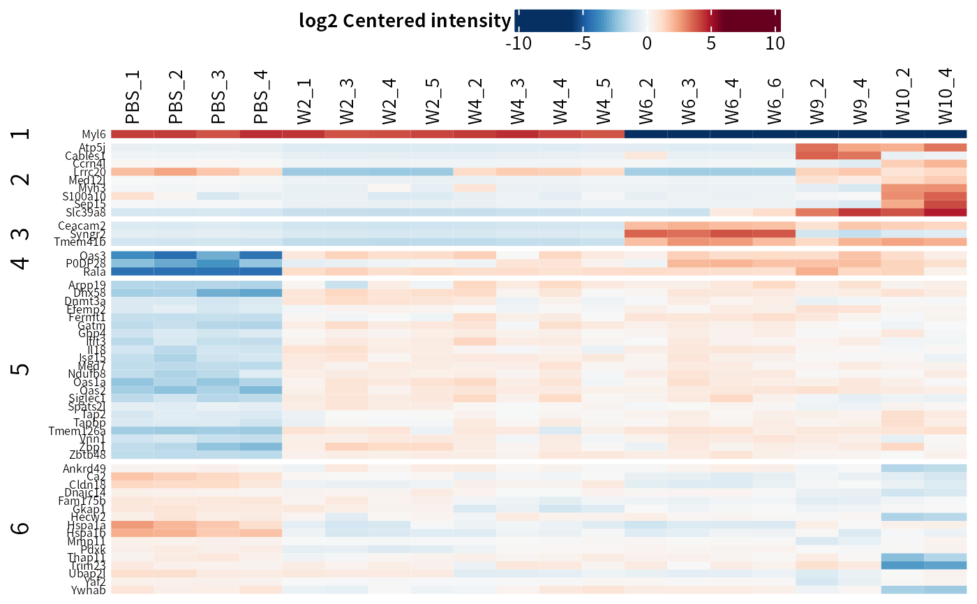
plot_heatmap can draw a ComplexHeatmap upon SE or DEGdata object out from add_rejections.
class(dep)
#> [1] "SummarizedExperiment"
#> attr(,"package")
#> [1] "SummarizedExperiment"

## Sort the conditions
dep = Order_cols(dep, order = c("PBS","W2","W4","W6","W9","W10"))

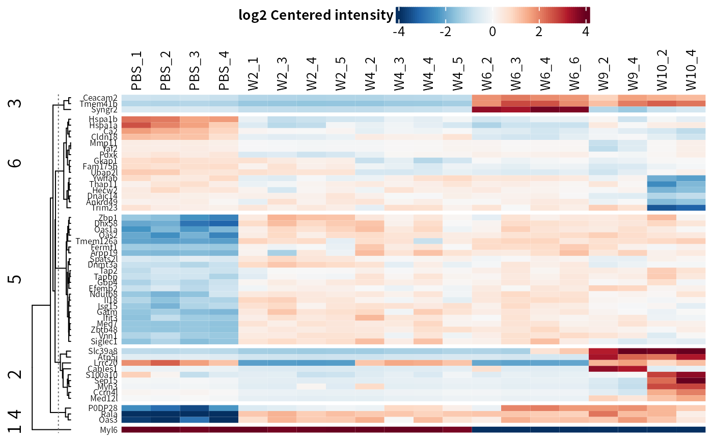
## Heatmap on centered values
DEP2::plot_heatmap(dep,
                   cluster_column = F,
                   kmeans = T,        # kmeans cluster rows
                   col_limit = 4      # limit of the color scale
) 
## Heatmap on contrast log2 foldchange
DEP2::plot_heatmap(dep,
                   type = "contrast",
                   cluster_column = F,
                   kmeans = T,
                   col_limit = 4)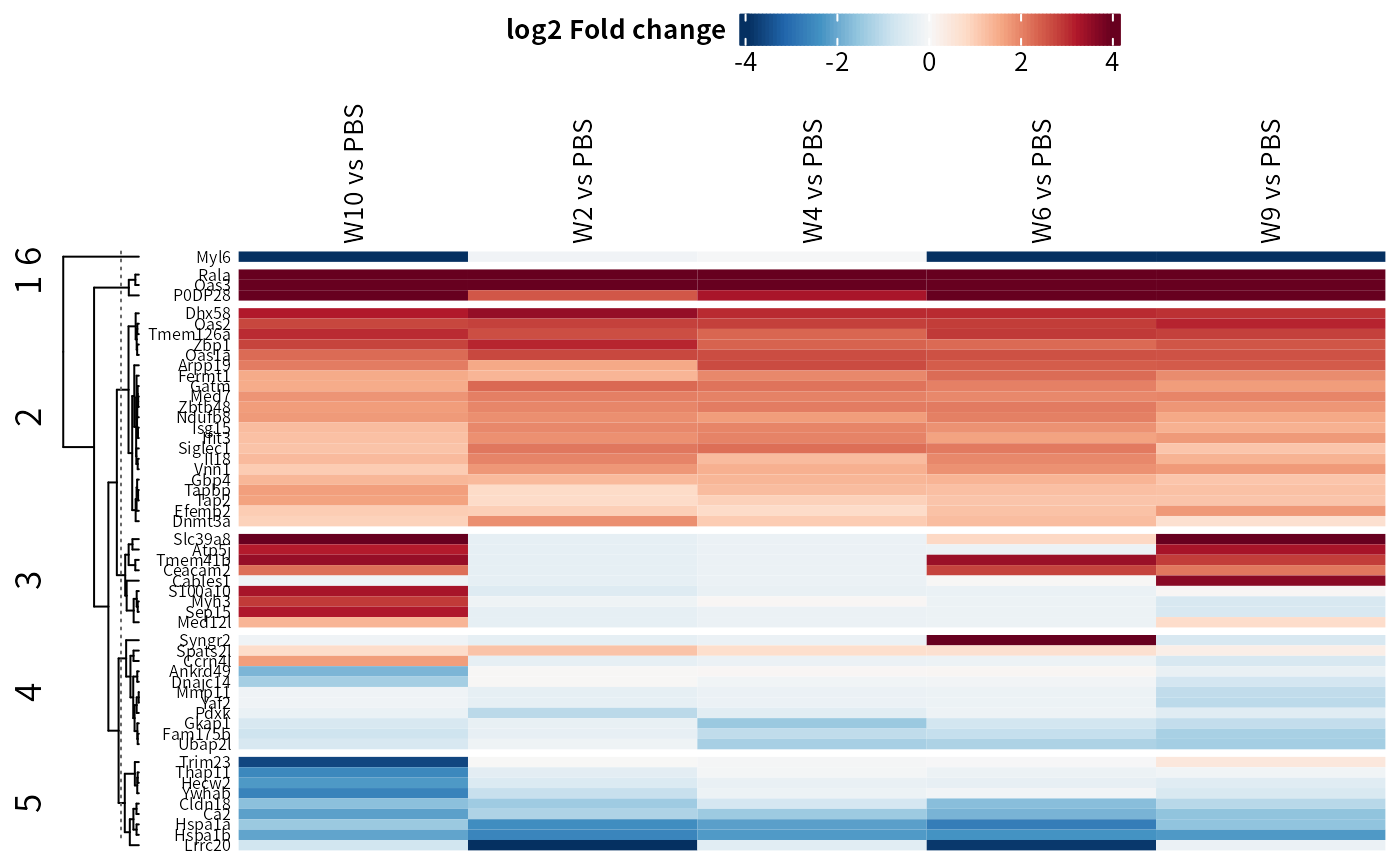
## Manual contrast
DEP2::plot_heatmap(dep,
                   manual_contrast = c("W6_vs_PBS","W4_vs_PBS"),
                   cluster_column = F,
                   kmeans = T,
                   col_limit = 4)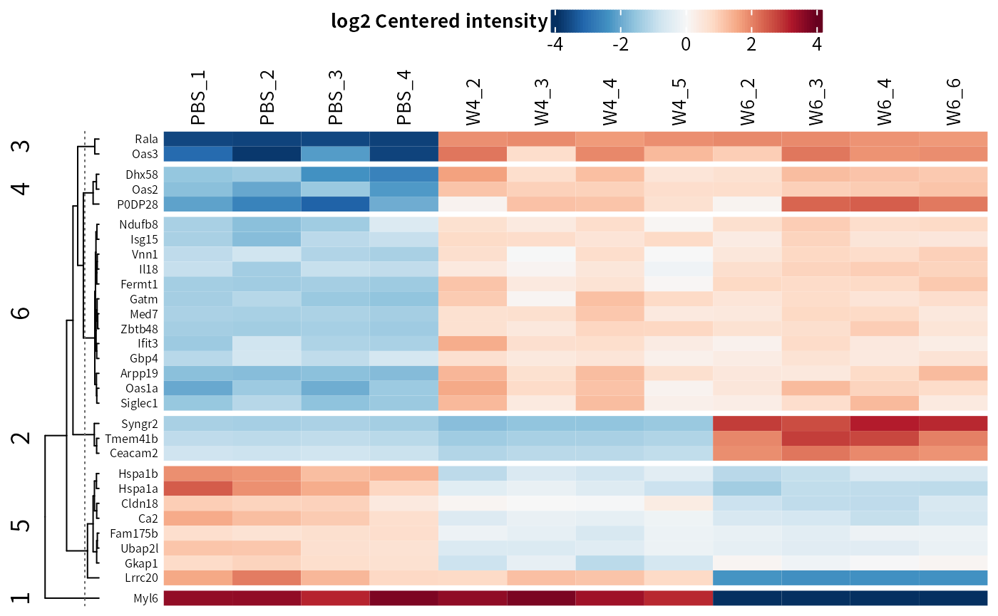
## Change color panel
DEP2::plot_heatmap(dep,
                   type = "contrast",
                   color = "PiYG",
                   cluster_column = F,
                   kmeans = T,
                   col_limit = 4)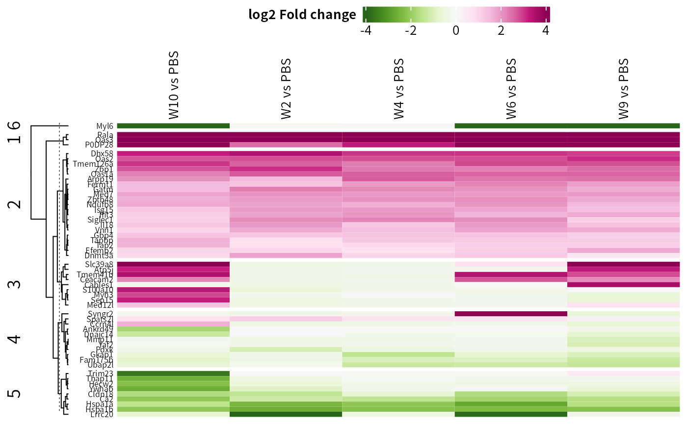
## Parameters in ComplexHeatmap::Heatmap are available
ht <- DEP2::plot_heatmap(dep,
                         cluster_column = F,
                         kmeans = T,
                         cluster_rows = F
                         )
## Heatmap can be saved as follow
# pdf("ht.pdf")
# ht
# dev.off()
Another common figure in omics study is the volcano plot, which can be created using plot_volcano.
plot_volcano(dep)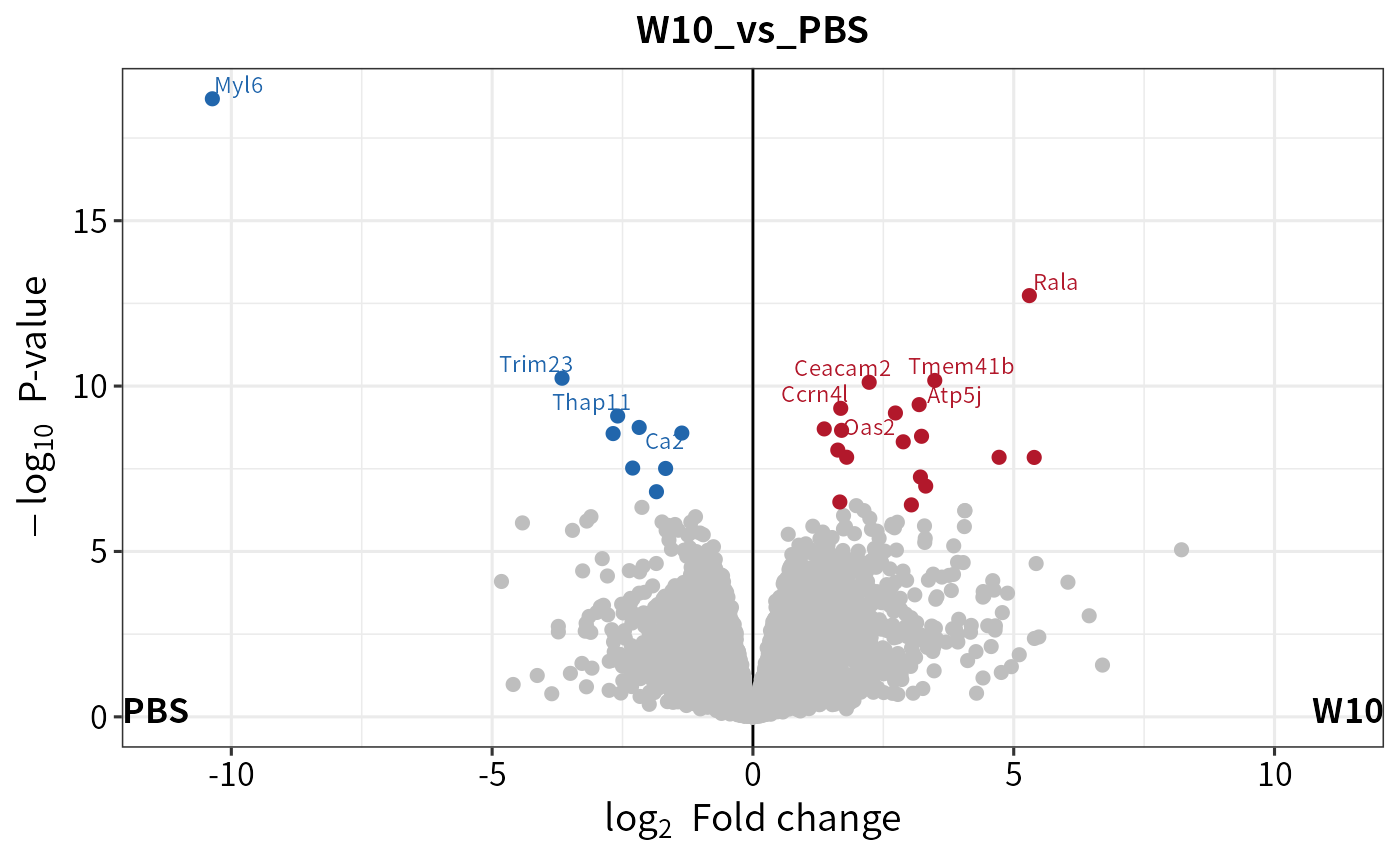
plot_volcano(deg,
             contrast = "W6_vs_PBS",  # contrast
             label_number = 20
             )
#> Warning: Removed 40 rows containing missing values (`geom_point()`).
#> Warning: ggrepel: 1 unlabeled data points (too many overlaps). Consider
#> increasing max.overlaps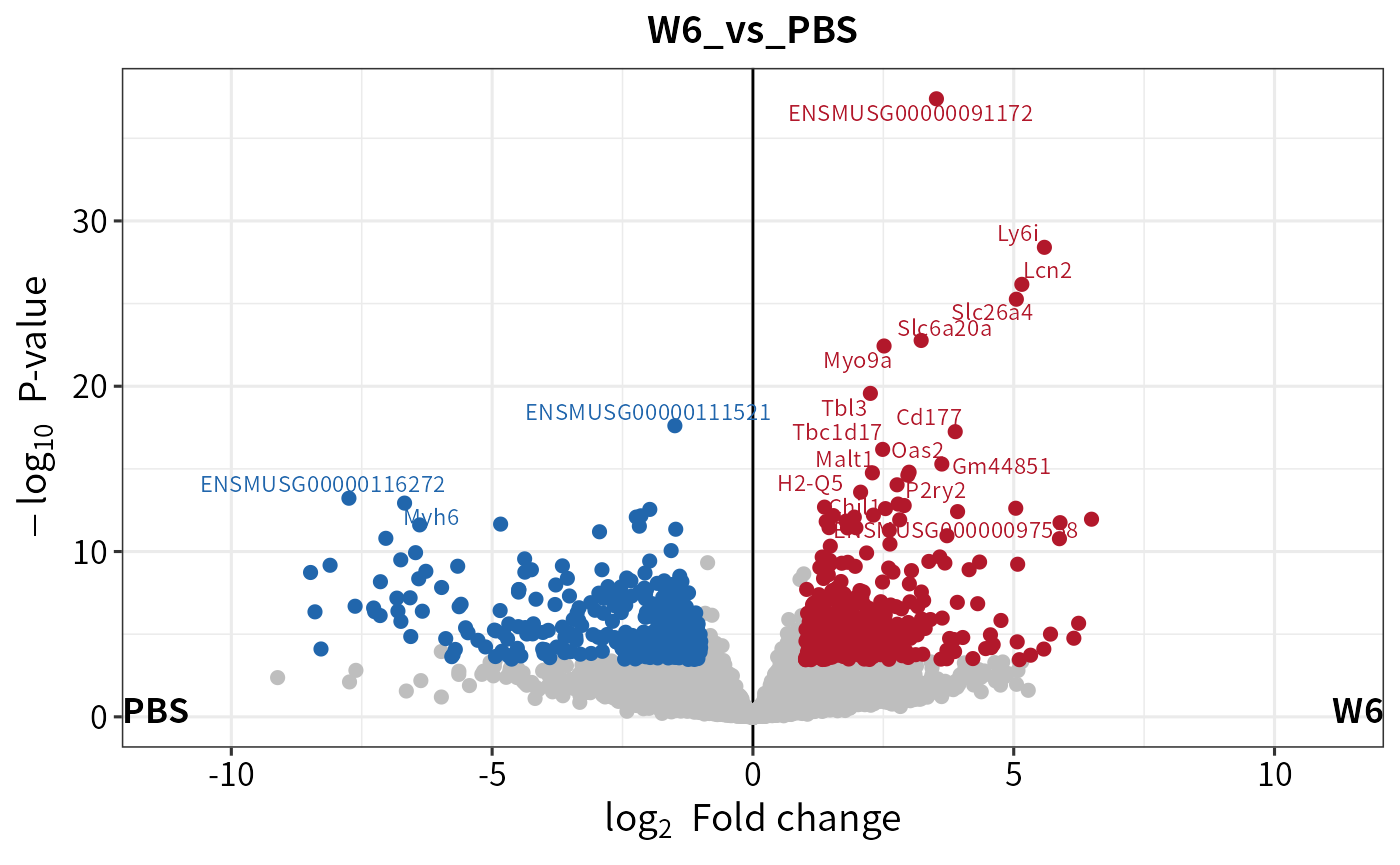
library(ggplot2)
(volc <- plot_volcano(deg, contrast = "W4_vs_PBS") + xlim(-10,10))
#> Scale for x is already present.
#> Adding another scale for x, which will replace the existing scale.
#> Warning: Removed 40 rows containing missing values (`geom_point()`).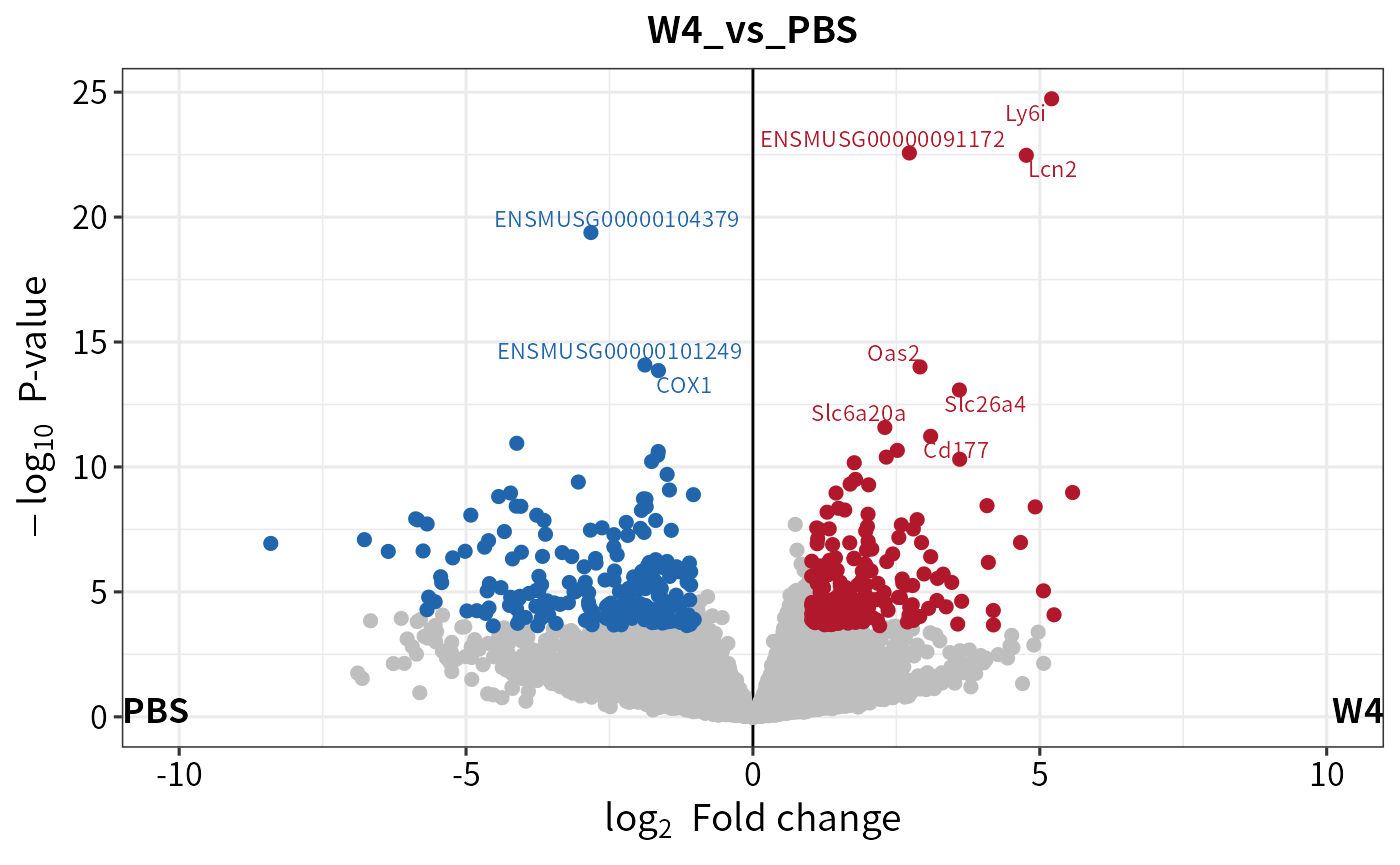
# ggplot2::ggsave(filename = "volcano.png") # export to fileExporting a table from an S4 object that inherits SE class is straightforward. Functions like SummarizedExperiment::colData and rowData can easily extract information from the object. DEP2 contains get_significant and get_df_wide to generate a significant result table or full dataset from the analysis result.
## Significant table
sig_tb <- get_signicant(dep,
                        return_type = "table"
                        )
sig_tb_W6_vs_PBS <- get_signicant(dep,
                                  return_type = "table" ,
                                  contrasts = "W6_vs_PBS"
                                  )

## Full table
full_tb <- get_df_wide(dep)

dim(sig_tb)
#> [1] 54 29
dim(sig_tb_W6_vs_PBS)
#> [1] 23 29
dim(full_tb)
#> [1] 9595   95

## Save table in R
# write.csv(full_tb,"fulldataset.cs",row.names = F)
Session information
#> R version 4.3.1 (2023-06-16)
#> Platform: x86_64-pc-linux-gnu (64-bit)
#> Running under: Ubuntu 18.04.5 LTS
#>
#> Matrix products: default
#> BLAS:   /usr/lib/x86_64-linux-gnu/blas/libblas.so.3.7.1
#> LAPACK: /usr/lib/x86_64-linux-gnu/lapack/liblapack.so.3.7.1
#>
#> locale:
#>  [1] LC_CTYPE=zh_CN.UTF-8       LC_NUMERIC=C
#>  [3] LC_TIME=zh_CN.UTF-8        LC_COLLATE=zh_CN.UTF-8
#>  [5] LC_MONETARY=zh_CN.UTF-8    LC_MESSAGES=zh_CN.UTF-8
#>  [7] LC_PAPER=zh_CN.UTF-8       LC_NAME=C
#>  [9] LC_ADDRESS=C               LC_TELEPHONE=C
#> [11] LC_MEASUREMENT=zh_CN.UTF-8 LC_IDENTIFICATION=C
#>
#> time zone: Asia/Shanghai
#> tzcode source: system (glibc)
#>
#> attached base packages:
#> [1] grid      stats4    stats     graphics  grDevices utils     datasets
#> [8] methods   base
#>
#> other attached packages:
#>  [1] org.Mm.eg.db_3.17.0         AnnotationDbi_1.62.2
#>  [3] ComplexHeatmap_2.16.0       ggplot2_3.4.2
#>  [5] dplyr_1.1.2                 DEP2_0.3.7.3
#>  [7] R6_2.5.1                    limma_3.56.2
#>  [9] MSnbase_2.26.0              ProtGenerics_1.32.0
#> [11] mzR_2.34.1                  Rcpp_1.0.11
#> [13] MsCoreUtils_1.12.0          SummarizedExperiment_1.30.2
#> [15] Biobase_2.60.0              GenomicRanges_1.52.0
#> [17] GenomeInfoDb_1.36.1         IRanges_2.34.1
#> [19] S4Vectors_0.38.1            BiocGenerics_0.46.0
#> [21] MatrixGenerics_1.12.2       matrixStats_1.0.0
#> [23] BiocStyle_2.28.0
#>
#> loaded via a namespace (and not attached):
#>   [1] splines_4.3.1               norm_1.0-11.1
#>   [3] bitops_1.0-7                tibble_3.2.1
#>   [5] lpsymphony_1.28.1           preprocessCore_1.62.1
#>   [7] XML_3.99-0.14               lifecycle_1.0.3
#>   [9] mixsqp_0.3-48               edgeR_3.42.4
#>  [11] doParallel_1.0.17           rprojroot_2.0.3
#>  [13] lattice_0.21-8              MASS_7.3-60
#>  [15] MultiAssayExperiment_1.26.0 magrittr_2.0.3
#>  [17] sass_0.4.6                  rmarkdown_2.23
#>  [19] jquerylib_0.1.4             yaml_2.3.7
#>  [21] doRNG_1.8.6                 askpass_1.1
#>  [23] reticulate_1.30             DBI_1.1.3
#>  [25] RColorBrewer_1.1-3          zlibbioc_1.46.0
#>  [27] Rtsne_0.16                  purrr_1.0.1
#>  [29] AnnotationFilter_1.24.0     itertools_0.1-3
#>  [31] RCurl_1.98-1.12             sandwich_3.0-2
#>  [33] circlize_0.4.15             GenomeInfoDbData_1.2.10
#>  [35] ggrepel_0.9.3               irlba_2.3.5.1
#>  [37] umap_0.2.10.0               RSpectra_0.16-1
#>  [39] missForest_1.5              pkgdown_2.0.7
#>  [41] ncdf4_1.21                  codetools_0.2-19
#>  [43] DelayedArray_0.26.6         tidyselect_1.2.0
#>  [45] gmm_1.8                     shape_1.4.6
#>  [47] farver_2.1.1                GenomicAlignments_1.36.0
#>  [49] jsonlite_1.8.7              GetoptLong_1.0.5
#>  [51] e1071_1.7-13                survival_3.5-5
#>  [53] iterators_1.0.14            systemfonts_1.0.4
#>  [55] bbmle_1.0.25                foreach_1.5.2
#>  [57] tools_4.3.1                 ragg_1.2.5
#>  [59] glue_1.6.2                  xfun_0.39
#>  [61] DESeq2_1.40.2               withr_2.5.0
#>  [63] numDeriv_2016.8-1.1         BiocManager_1.30.21
#>  [65] fastmap_1.1.1               fansi_1.0.4
#>  [67] openssl_2.0.6               digest_0.6.33
#>  [69] truncnorm_1.0-9             imputeLCMD_2.1
#>  [71] textshaping_0.3.6           colorspace_2.1-0
#>  [73] RSQLite_2.3.1               utf8_1.2.3
#>  [75] tidyr_1.3.0                 generics_0.1.3
#>  [77] data.table_1.14.8           class_7.3-22
#>  [79] httr_1.4.6                  S4Arrays_1.0.4
#>  [81] pkgconfig_2.0.3             gtable_0.3.3
#>  [83] blob_1.2.4                  impute_1.74.1
#>  [85] XVector_0.40.0              htmltools_0.5.5
#>  [87] bookdown_0.34               MALDIquant_1.22.1
#>  [89] clue_0.3-64                 scales_1.2.1
#>  [91] tmvtnorm_1.5                png_0.1-8
#>  [93] ashr_2.2-54                 knitr_1.43
#>  [95] rstudioapi_0.15.0           reshape2_1.4.4
#>  [97] rjson_0.2.21                coda_0.19-4
#>  [99] bdsmatrix_1.3-6             proxy_0.4-27
#> [101] cachem_1.0.8                zoo_1.8-12
#> [103] GlobalOptions_0.1.2         stringr_1.5.0
#> [105] parallel_4.3.1              mzID_1.38.0
#> [107] vsn_3.68.0                  desc_1.4.2
#> [109] apeglm_1.22.1               pillar_1.9.0
#> [111] vctrs_0.6.3                 pcaMethods_1.92.0
#> [113] slam_0.1-50                 randomForest_4.7-1.1
#> [115] IHW_1.28.0                  cluster_2.1.4
#> [117] evaluate_0.21               magick_2.7.4
#> [119] invgamma_1.1                mvtnorm_1.2-2
#> [121] cli_3.6.1                   locfit_1.5-9.8
#> [123] compiler_4.3.1              Rsamtools_2.16.0
#> [125] rlang_1.1.1                 crayon_1.5.2
#> [127] rngtools_1.5.2              SQUAREM_2021.1
#> [129] labeling_0.4.2              fdrtool_1.2.17
#> [131] TCseq_1.23.0                emdbook_1.3.13
#> [133] QFeatures_1.10.0            affy_1.78.1
#> [135] plyr_1.8.8                  fs_1.6.2
#> [137] stringi_1.7.12              BiocParallel_1.34.2
#> [139] assertthat_0.2.1            munsell_0.5.0
#> [141] Biostrings_2.68.1           lazyeval_0.2.2
#> [143] glmnet_4.1-7                Matrix_1.5-4.1
#> [145] bit64_4.0.5                 KEGGREST_1.40.0
#> [147] highr_0.10                  igraph_1.5.0
#> [149] memoise_2.0.1               affyio_1.70.0
#> [151] bslib_0.5.0                 bit_4.0.5
#> [153] downloader_0.4